Although transonic flight is now commonplace, new, nonconventional designs are being proposed and evaluated. As such, transonic testing is still a topic of interest. One type of test facility that allows transonic flows at high Reynolds number is a Ludwieg tube tunnel. These tunnels have short test times of about 0.1 s. While force measurements have proceeded in a conventional manner, recent developments in dynamic force measurements in hypersonic shock tunnels have led the same principles to be applied by Werling. Werling performed experiments on a transonic NACA 0012 wingtip. The force measurement was corrected for dynamic effects arising from stress waves propagating through the model/balance structure. The present work is to validate the experimental force coefficients via numerical simulations. The numerical approach uses NASA’s FUN3D (Fully-Unstructured Navier-Stokes 3D) flow solver.
Because the analyst cannot specify a velocity profile at the inlet within the FUN3D framework, an inverse problem is solved to determine the correct length of the test section so that the boundary layer grows to the appropriate size (as determined by previous experiments). Pointwise is used to parameterize and generate the geometry. Pointwise tasks can be scripted using an internal programming language called Glyph which is based on Tcl. After generating the surface grids using Pointwise, the volume grids are generated using AFLR3. The entire process is automated using the Python scripting language. The optimization tools in the SciPy package are used to solve the inverse problem.
Preliminary contours of pressure coefficient on the upper surface of the wing at α = 4 deg are shown in Fig. 3 and a comparison between experimental and CFD surface flow visualization is shown in Fig. 4. While the comparison is not exact, similarities between the two figures are encouraging. Shock induced boundary layer separation is evident in both figures. The Mach 1 isosurfaces in Fig. 5 and Fig. 6 show the transonic flow over the top of the airfoil. The back side of the isosurface shows the shock location. The final paper will include results from solving the inverse problem as well as a comparison between CFD and experiment. The data compared will include force coefficients and a comparison of flow separation zones. Further 3D flow details from CFD that are difficult to obtain from experiment will be reported.
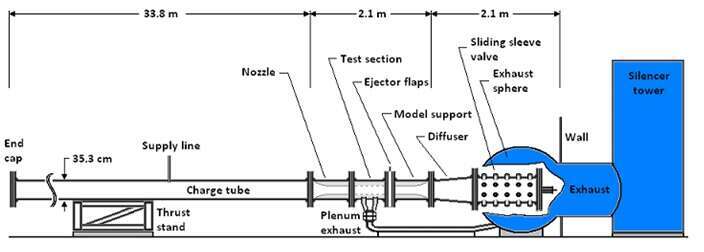
Figure 1. Schematic of transonic Ludwieg tube tunnel.
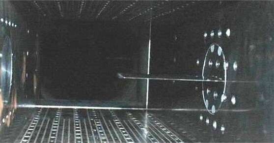
Figure 2. Test section showing wingtip.
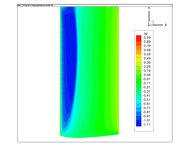
Figure 3. Preliminary contours of pressure coefficient of upper surface at α=4 deg; flow from left to right.
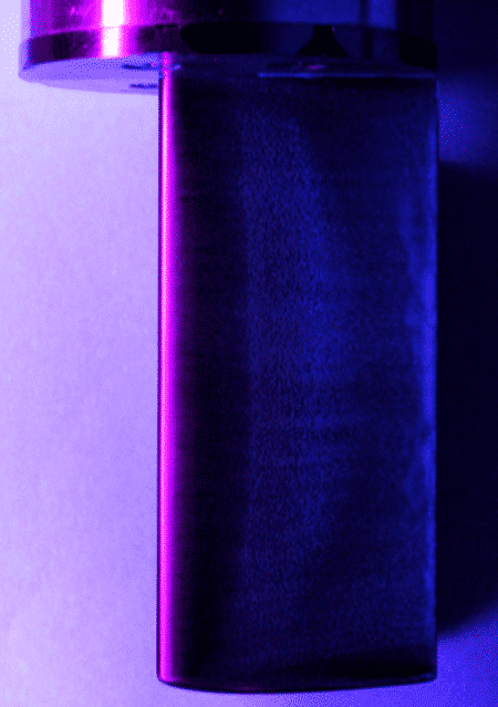
Figure 4(a). Experimental surface flow visualization of upper surface at α=4 deg; flow from left to right.
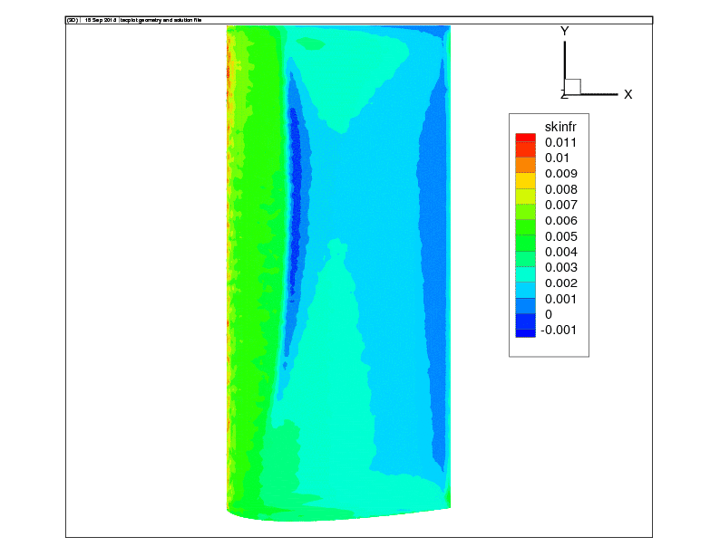
Figure 4(b). CFD surface flow visualization of upper surface at α=4 deg; flow from left to right.
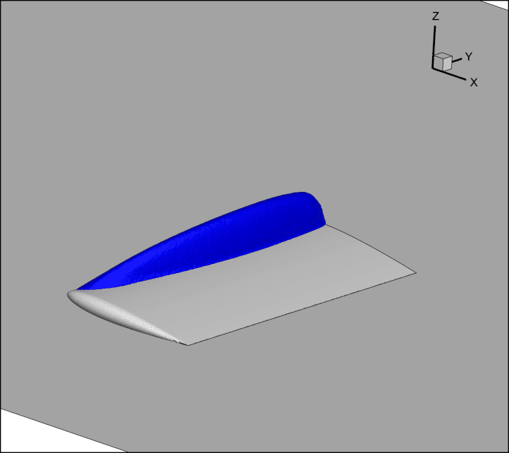
Figure 5. Mach 1 isosurface; flow from top left to bottom right.
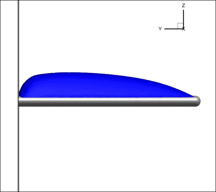
Figure 6. Mach 1 isosurface (front view).
